AI for Logistics and Supply Chain
AI for logistics and supply chain, built on the data you already have.
Late shipments, carrier rate surprises, warehouse inefficiency, and demand forecasts built in spreadsheets: these are operations problems that AI can reduce. The question is which problem to solve first and what data you already have to work with.
We build AI systems for logistics and supply chain operations: demand forecasting models, route optimization, predictive ETAs, carrier rate prediction, exception detection, document extraction from shipping documents, and load optimization. Every system is scoped against your data and a specific operational outcome.
Demand forecasting models that reduce overstock and stockout simultaneously
Predicted ETAs and delay alerts before the customer asks where their shipment is
Carrier rate prediction so procurement buys at the right time, not the wrong time
Document extraction from BOLs, PODs, customs forms, and invoices without manual re-keying
Bring the problem, the current workflow, or the existing code. We reply with a practical next step within one business day.
Trusted by
































The brief
Start with what is not working.
Good software decisions begin with the constraint, not a list of features or a preferred technology.
01
Are your demand forecasts consistently off by enough margin to cost you either carrying costs or lost sales?
02
Are you finding out about shipment exceptions at the same time your customer does?
Plain answer
RaftLabs builds AI systems for logistics and supply chain operations across the US, UK, Europe, Canada, and the UAE: demand forecasting, route optimization, predictive ETAs, carrier rate prediction, exception detection, and shipping document extraction. McKinsey ties AI-enabled supply chains to 5-20% lower logistics costs. Projects run 12 weeks at a fixed price.
What to remember
- RaftLabs builds AI systems for logistics and supply chain operations across the US, UK, Europe, Canada, and the UAE, covering demand forecasting, route optimization, predictive ETAs, carrier rate prediction, exception detection, and shipping document extraction.
- Projects run 12 weeks at a fixed price, with most logistics AI engagements ranging from $30,000 to $120,000 depending on scope.
- McKinsey ties AI-enabled supply chain operations to 5-20% lower logistics costs, 20-30% lower inventory, and 20-50% smaller forecast error versus conventional methods.
- A multi-carrier shipping platform migrated 200+ existing customers with zero service disruption and handled 2,000+ shipments across 70+ countries in year one.
The delay was predictable. Your system just didn't say so.
A shipment leaves the dock on a carrier that runs late on this lane this time of year. The weather ahead is turning, and the scan events are already spacing out. Every signal that predicts a late delivery is present at booking.
Most operations still find out about the exception at the same moment the customer does. The information to predict it was usually there. The question is whether your system acts on it.
Finding out about a delay when your customer does is not a system failure. It is a data and model failure.
Late shipments, carrier rate surprises, warehouse inefficiency, and demand forecasts built in spreadsheets are operations problems that AI can reduce. The question is which problem to solve first, and what data you already have to work with. We build AI systems for logistics and supply chain operations: demand forecasting models, route optimization, predictive ETAs, carrier rate prediction, exception detection, document extraction from shipping documents, and load optimization. Every system is scoped against your data and a specific operational outcome.
Supply chain AI is most valuable when it moves your operation from reactive to anticipatory. According to McKinsey, AI-enabled supply chain operations deliver 5-20% logistics cost reduction, 20-30% inventory reduction, and 5-15% procurement spend reduction compared to conventional methods, and AI-based forecasting cuts error rates 20-50% against traditional methods. For logistics operators, those numbers trace directly to demand forecasting accuracy, exception detection speed, and carrier rate timing: the three levers that compound fastest.
Which system to build first is a scoring question, not a taste question. We rank your candidate use cases on two axes: how ready the data is, and how much the outcome moves your P&L. The one that scores high on both ships first. That ranking is the output of week-one discovery, before anyone trains a model.
AI pays off when you have data and a specific outcome to point it at.
Everything on the left should already be true for your operation. Even one thing on the right, and scoping the data comes before any model.
A fit
01
18-36 months of historical order, shipment, or rate data to train a model on.
02
A specific operational problem to measure against: late deliveries, forecast inaccuracy, excess carrier spend, or document processing time.
03
A TMS, ERP, or WMS the model can integrate with via API.
Not a fit
01
No historical data yet, or data you cannot export from your current systems.
02
You want an off-the-shelf tool, not a system scoped to your operation.
03
No specific operational outcome to benchmark the model against.
What we build
Systems we build for logistics and supply chain
- 01
Demand forecasting models
Demand forecasting models trained on your historical order data, typically 18-36 months of line-item history at SKU and location level, with architecture matched to your data. Promotional calendars, pricing history, and weather feed the feature set, and output is a daily or weekly forecast per SKU per location with P10/P50/P90 intervals, benchmarked against your current method before deployment. Built on LightGBM, XGBoost, Temporal Fusion Transformer, and Prophet. - 02
Route optimization
Route optimization using a Vehicle Routing Problem with Time Windows solver augmented with ML-predicted travel times from live traffic, historical patterns, and weather. Routes re-optimize every 30-60 minutes as conditions, driver locations, and new orders change, with constraints covering vehicle capacity, customer time windows, hours of service regulations, and vehicle compatibility, delivered to your TMS via REST API. Built on a VRPTW solver with Oracle TMS, SAP TM, and project44 integration. - 03
Predictive ETA and exception detection
Predictive ETA and exception detection models score each in-transit shipment at booking and update the risk as new data arrives, using features like carrier on-time history per lane, scan event gaps, and route weather. Output is a delay probability and a P25/P50/P75 delivery range, and high-risk shipments surface to the exception queue with plain-language risk factors so automated customer notifications go out before the customer calls. - 04
Carrier rate prediction
Carrier rate prediction models forecast spot and contract rate movements for specific lane-mode combinations at weekly and monthly horizons, using inputs like diesel price indices, spot rate history, tender acceptance rates, and seasonal demand. Output is a lane-specific forecast with a confidence range and a buy-now-or-wait signal, backtested against your own rate transactions before deployment. Fed by DAT spot rates, the Freightos Baltic index, and diesel price indices. - 05
Shipping document extraction
Shipping document extraction uses OCR plus LLM-based extraction to parse structured data from the varying formats of logistics documents: bills of lading, proof of delivery, customs entries, and freight invoices. Documents are classified by type, read, then normalized into structured output, with low-confidence fields queued for human review and results delivered via API to your TMS or ERP. Built on Azure Document Intelligence, AWS Textract, GPT-4o, and Claude. - 06
Load and warehouse slotting optimization
Load optimization solves the 3D bin-packing and weight-distribution problem to maximize trailer utilization and ensure legal axle weight compliance, with stackability, hazmat segregation, and multi-stop loading constraints built in. A 5-12% utilization improvement on mixed freight is common, and warehouse slotting analysis mines your WMS pick history to rank slot moves by expected pick travel reduction, re-running monthly or quarterly as velocity patterns shift. - 07
Voice-directed picking and dispatch
Hands-free voice agents for warehouse pick confirmation, shipment status calls, and driver dispatch coordination, built on transcription models tuned for high-noise warehouse and in-cab acoustics rather than general-purpose speech recognition. Warehouses moving from paper or scan-based picking to voice-directed operations typically cut pick error rates by 20 to 35 percent within 90 days. Built on Deepgram noise-tuned transcription models.
Which logistics problem costs you the most right now?
Bring us the specific operational problem: late deliveries, forecast inaccuracy, excess carrier spend, or document processing time. We'll assess whether AI reduces it and what it costs to build.
How it works
From scope to shipped
Every project follows the same four phases. Scope is locked and price is fixed before development starts.
- Week 101
Discovery and data audit
We map the operational problem, the data you have, and the accuracy improvement that is realistic. You leave week 1 with a written scope document and a fixed-price quote. No development starts without your sign-off.
- Weeks 2-302
Model design and architecture
We select the model architecture based on your data characteristics and the target output. Feature engineering, training pipeline design, and evaluation metrics are locked before the build starts.
- Weeks 4-1203
Build, train, and integrate
Model trained and evaluated against your historical data by sprint 1. API integration into your TMS, ERP, or WMS follows. QA runs in parallel with every sprint, not as a phase at the end.
- Weeks 12+04
Deploy and monitor
Production deployment with model performance monitoring activated on launch day. Drift detection alerts when model accuracy degrades. 8 weeks of post-launch support included in every project.
Proof
Case studies
AI OCR for gas station operations

IntroJoy reaches 10,000 users in 6 months by replacing the email chain with a structured double opt-in introduction flow
IntroJoy removes the back-and-forth from warm professional introductions. Both parties confirm via double opt-in email, the connector is done after drafting once, and professional networks grew 20% for active users.
Most logistics AI projects run between $30,000 and $120,000. Where you land depends on scope, not negotiation:
- Focused build
- A document extraction system for a single document type, sitting at the lower end of the range.
- Larger scope
- A demand forecasting model covering 5,000 SKUs across 10 locations with external signal integration.
What it costs
Logistics AI, starting at $30,000.
Every system is scoped against your data and a specific operational outcome in a paid discovery engagement, then built at a price locked before work starts.
We scope one system first in a paid discovery engagement and price it. The results make the case for whether the next one is worth building.
Starting investment
Starts at $30,000
12 weeks to production for the first system, with 8 weeks of post-launch support included. Most operators start with one system and add the next once it's proven.
No hourly billing
We scope the work, calculate the cost, and lock it in writing before any development starts. No hourly billing. A scope change is a change request: priced, agreed, or dropped, never absorbed into the project.
Support and monitoring
8 weeks of post-launch support is included in every project, with model performance monitoring and drift detection active from launch day.
Useful next steps
More on logistics & fleet
Work with us
Work with us
Inventory Management ERP
See the serviceTry it yourself
Try it yourself
Logistics Software Cost Calculator
TMS, fleet, freight, or shipping software. Honest build range in 3 minutes.
Open the free tool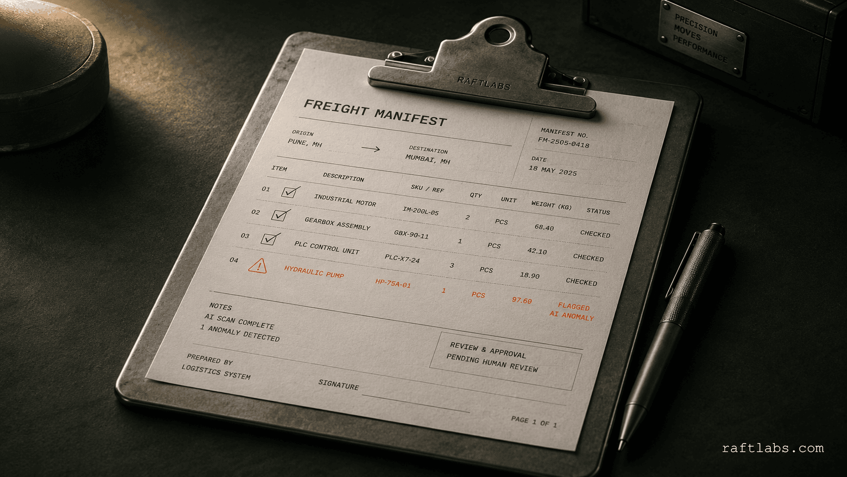
Article
AI in Logistics: Cutting Costs on Thin Margins
Logistics runs on margins that leave no room for inefficiency. Carriers, fuel, dwell time, customs delays, every friction point is a cost that compounds across millions of shipments. AI addresses each of these, but not equally. Here is where the numbers actually justify the investment.
Read more
Article
Towing Dispatch Software: Build vs. Buy for Fleet Operators
TowBook and Dispatch.Me handle basic jobs fine. When you run 15+ trucks, multiple motor clubs, and impound lots across locations, off-the-shelf towing dispatch software stops working. Here is what custom towing management software development actually costs, how long it takes, and when it makes sense.
Read more
Article
How much does IoT development cost? (2026 breakdown)
An IoT system costs $20,000-$300,000+ to build depending on device complexity, connectivity type, and fleet size. Here's what drives the range, three real budget scenarios, and what ongoing costs look like in production.
Read more
Article
Intelligent Document Processing for Logistics and Supply Chain
Intelligent document processing for logistics automates bills of lading, POD matching, vendor contracts, and warehouse inventory records, reducing freight delays.
Read moreCommon questions
A demand forecasting model needs historical order or sales data, typically 18-36 months minimum, with enough granularity to detect seasonality and trend. Beyond the base demand history, the model improves significantly when you add external signals: promotional calendars (what promotions ran when), inventory availability history (was a stockout driven by demand or supply?), pricing history, and where relevant, external signals like weather data, economic indicators, or commodity prices. The model architecture we choose depends on the data you have. For most logistics and distribution businesses, a gradient boosting model or a temporal fusion transformer trained on your order history gives meaningfully better accuracy than a statistical forecast from a spreadsheet. We assess your data in discovery and tell you what accuracy improvement is realistic before we build.
Exception prediction is a classification problem. A model is trained on historical shipment data: shipments that completed on time, and shipments that experienced delays, damaged goods, missing documentation, or carrier failures. The model learns which combinations of signals, carrier, lane, origin-destination pair, time of year, weather conditions, shipment weight and dimensions, and days in transit, predict exceptions before they happen. At the point of booking or during in-transit monitoring, each shipment is scored. High-risk shipments are surfaced to your operations team with the contributing risk factors so they can intervene: hold alternatives ready, alert the customer proactively, or escalate with the carrier before the exception becomes a miss. The key difference from reactive tracking is that the alert comes before the delay is confirmed, not after.
Warehouse slotting is the assignment of SKUs to pick locations based on velocity, pick frequency, and co-order patterns. A poorly slotted warehouse has pickers traveling long distances for high-velocity items and fast-moving SKUs stored in inconvenient locations. Traditional slotting uses velocity-based rules: A, B, and C items by pick frequency. AI-based slotting adds co-order analysis, which identifies SKUs that are frequently picked together in the same order and places them near each other, and temporal patterns, which identify how velocity changes by day of week, month, or season. The output is a recommended slot assignment that reduces total pick distance and therefore pick time per order. For high-volume operations, slotting optimization typically reduces pick travel distance by 15-30%. We build this as a model that runs against your WMS data on a scheduled basis and produces re-slot recommendations, not as a one-time exercise.
Standard TMS routing solves the vehicle routing problem using rules-based optimization: minimize distance or time given a set of stops and vehicle constraints. This works well for predictable, static conditions. AI-based route optimization adds two capabilities standard TMS tools lack. First, it incorporates real-time signals: live traffic conditions, weather, road incidents, and driver performance history. It re-optimizes routes dynamically as conditions change, not just at the start of the day. Second, it learns from historical outcomes: which routes resulted in late deliveries, which drivers perform better on specific lane types, which stop sequences cause driver overtime. Over time, the model improves its routing quality because it learns from your specific operation rather than applying generic optimization rules. For fleets running 50 or more routes per day, the combination of dynamic re-optimization and learned performance patterns typically reduces fuel cost and late deliveries meaningfully. We scope the specific impact against your data during discovery.
Most logistics AI projects with RaftLabs run between $30,000 and $120,000 depending on scope. A focused document extraction system for a single document type typically sits at the lower end. A demand forecasting model covering 5,000 SKUs across 10 locations with external signal integration is a larger scope. We scope the work in a paid discovery engagement before any development starts, then give you a fixed-price quote. The price you see in week 1 is the price on the final invoice, unless you change the scope.
Voice-directed picking delivers task instructions through a headset and takes verbal confirmation before advancing to the next task, so workers stay mobile instead of stopping to read a screen or a paper list. This eliminates the misread-screen and illegible-paper-list errors that drive most pick mistakes. Warehouses transitioning from scan-based picking typically see error rates drop 20 to 40 percent within 90 days. Deepgram's noise-tuned transcription models are essential here, general-purpose speech recognition performs poorly against conveyor noise, forklift traffic, and PA announcements, while warehouse-tuned models hold word error rates below 3 percent in the same conditions.
Yes. We sign mutual NDAs before any scoping conversation where you share operational data, pricing data, or proprietary processes. For enterprise logistics clients, we are open to signing your standard NDA form rather than asking you to use ours. Confidentiality extends to your data: model training data is used only to train your model and is not shared across client accounts or used in any way outside your project.
Work with us
Tell us where the work is stuck.
Bring the rough workflow, half-built product, or messy brief. We will map the smallest useful first move, then send scope, timeline, and price in plain English.
- Scope and cost agreed before work starts. No surprises. No obligation.
- Working prototype within 3 weeks of kickoff.
- Pay by milestone. You see progress before each invoice.
- 60-day post-launch warranty. Bug fixes, UI tweaks, and deployment support. No retainer.
- All conversations are NDA-protected.