
Charles E.
Entrepreneur at Aggie Technologies
 USA
USA
All of the sprints were completed on schedule and on budget. We highly recommend RaftLabs!
AI for Energy and Utilities
Equipment failures that weren't predicted, grid imbalances found after the fact, and field technicians dispatched reactively: these are the operational costs that AI reduces in energy and utilities. The sensor and meter data to prevent them already exists in most operations.
We build AI systems for utilities, energy companies, and oil and gas operators: predictive maintenance for generation and distribution assets, demand forecasting for grid management, anomaly detection for pipeline and grid infrastructure, AI field service routing, energy consumption optimization for buildings, renewable energy output forecasting, and AI-driven customer billing anomaly detection. Every system is scoped against your operational data and a specific asset or cost target.
Predictive maintenance models that surface asset failure risk weeks before a trip or outage occurs
Demand forecasts at the feeder and substation level that reduce both reserve costs and grid imbalances
Anomaly detection on SCADA and pipeline sensor data that flags deviations before they become incidents
Renewable output forecasts that improve dispatch decisions and reduce curtailment costs
Bring the problem, the current workflow, or the existing code. We reply with a practical next step within one business day.
Trusted by































The brief
Good software decisions begin with the constraint, not a list of features or a preferred technology.
Are your maintenance teams responding to equipment failures after they happen, or do you have a model that surfaces failure risk before it trips?
Are your grid demand forecasts accurate enough to optimize reserve procurement, or are you carrying excess reserve to cover forecast uncertainty?
Plain answer
RaftLabs builds AI for energy and utilities across the US, UK, Europe, Canada, GCC, South Africa, and Southeast Asia: predictive maintenance, demand forecasting, pipeline anomaly detection, and renewable output forecasting. Each engagement is fixed-price after a discovery week that maps your SCADA data to a specific cost target.
What to remember
A transformer trips on a Tuesday afternoon. The crew is dispatched after the outage, the load is shed, and the post-mortem finds the oil temperature had been drifting for weeks. Every signal was there, in the SCADA historian, unread.
Predictive maintenance reads them first. The same sensor stream, scored daily, surfaces the asset weeks before it trips, ranked by failure probability with the contributing signals attached. The maintenance team plans the intervention instead of reacting to the outage.
The data was never the problem. Nobody was listening to it.
Energy AI is most valuable when it moves your operations team from reacting to failures to anticipating them. The sensor data to predict most equipment failures already exists in your SCADA and monitoring systems. The question is whether a model is turning that data into actionable maintenance signals.
According to Gartner's January 2025 outlook, 94% of power and utility CIOs plan to increase AI investments in 2025, with an average spending increase of 38.3%, and 40% of utilities are expected to deploy AI-driven operators in control rooms by 2027. The investment is accelerating because operations teams are proving ROI on specific asset classes first, then expanding the model footprint.
RaftLabs has shipped production software since 2015 for clients across the US, UK, Europe, Canada, and the UAE. NERC CIP, FERC, and GDPR requirements are scoped in week 1, not retrofitted before launch, and the team that scopes your build ships it, from kick-off to a production-ready system in about 12 weeks.
Everything on the left should already be true for your operation. Even one thing on the right, and a scoping conversation comes before any build.
You run generation, distribution, pipeline, or renewable assets with sensor and meter data already flowing into a SCADA system or historian.
You have a specific asset class or cost target in mind: transformer failures, reserve procurement, pipeline anomalies, or curtailment.
You have 2-3 years of historical load, sensor, or failure records for a model to learn from.
Your sensor and meter data isn't captured or accessible yet.
You want a generic AI pilot with no asset class or cost target attached.
You need an off-the-shelf dashboard, not a model trained on your operational data.
What we build
We build AI systems that optimize HVAC and building load using occupancy data, sub-metering, weather inputs, and tariff structure. The model manages pre-conditioning and demand peak shaving to reduce both energy consumption and demand charges. For building operators or energy service companies managing a portfolio of commercial assets, the same model architecture runs across all buildings with asset-specific calibration.
Maintenance surprises, forecast inaccuracy, or pipeline anomalies: tell us the specific operational problem and we will assess which AI system addresses it and what your sensor data supports.
How it works
Every project follows the same four phases. Scope is locked and price is fixed before development starts.
We map the problem, the asset class, and your sensor data availability. You leave week 1 with a written scope document and a fixed-price quote. No development starts without your sign-off.
We build a prototype model against a sample of your historical data and validate prediction quality before committing to the full build. If the data doesn't support the use case, you know in week 3, not week 12.
Working AI system at a staging environment by the end of sprint one. Bi-weekly demos. Integration into your SCADA, CMMS, or BMS runs in parallel with model development.
Production deployment with monitoring activated on launch day. 8 weeks of post-launch support included. Model drift detection flags when retraining is needed.
What clients say
Three-year average engagement. Founders and operators describing the work in their own words. No marketing varnish.
Charles E.
Entrepreneur at Aggie Technologies
USA
All of the sprints were completed on schedule and on budget. We highly recommend RaftLabs!
01 / 02
Proof

We helped Snelweg Deals move from offline vehicle resale to a digital marketplace with a guided seller form, real-time dealer bidding, Dutch number plate lookup via the Overheid API, and automated invoicing through Moneybird.
Every engagement is fixed-price after a discovery week. Where you land depends on scope, not negotiation:
What it costs
A focused model for a single asset class, or a multi-system platform across demand forecasting, anomaly detection, and field service routing. Both are scoped against your operational data and a specific cost target.
Most operators start with one asset class, validate the model against real sensor data, then expand to the next system.
Starting investment
Starts at USD 40,000
Covers a focused predictive maintenance model for one asset class. Multi-system platforms are scoped and priced after a discovery week, once the first model has proven itself.
No hourly billing
We map the problem, the asset class, and your sensor data availability, then lock the price in writing. No hourly billing and no development starts without your sign-off. A scope change is a priced change request.
Validate first
We build a prototype against a sample of your historical data and validate prediction quality in week 3. If the data doesn't support the use case, you know then, not in week 12.
Useful next steps
Work with us
Solar Monitoring Software Development
See the service
Article
AI for manufacturing: From predictive maintenance to quality control
Your factory floor runs on SCADA and PLCs. Your business runs on ERP and MES. AI agents bridge that gap - taking autonomous action across both systems without the 18-month integration project.
Read more
Article
Online Car Buying Platform Development: Cost, Timeline, and What You Actually Need
Auto dealers and used car marketplaces paying $1,500-$3,000 per lead to Carvana and CarGurus can build their own online car buying platform for $80K-$140K in 16-20 weeks. Here is exactly what that covers, where clone scripts fail, and who should build one.
Read more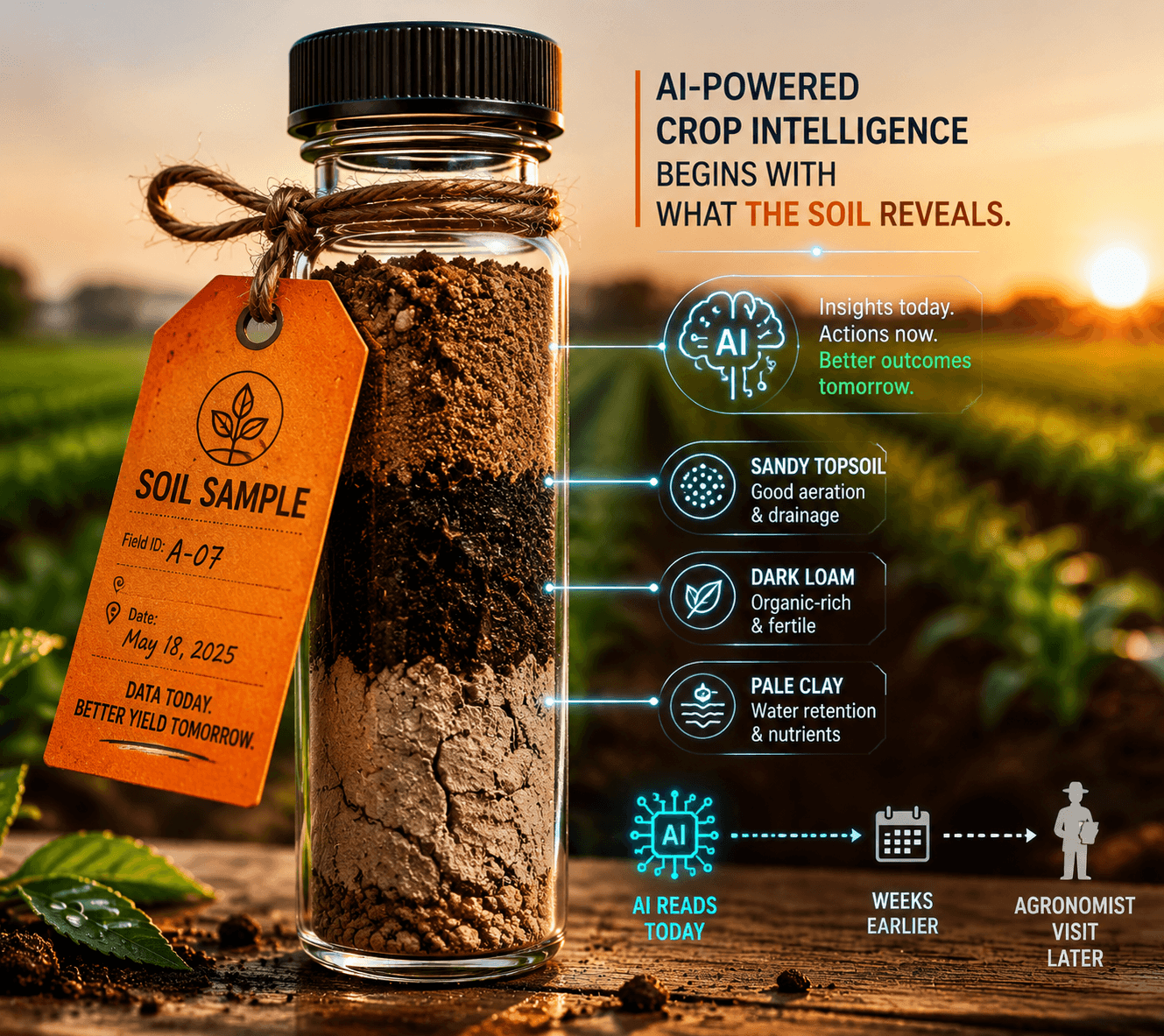
Article
AI in agriculture: What's working in 2026
Plant diseases cost the industry $220B a year. AI agents are catching them weeks earlier - without waiting for an agronomist visit.
Read more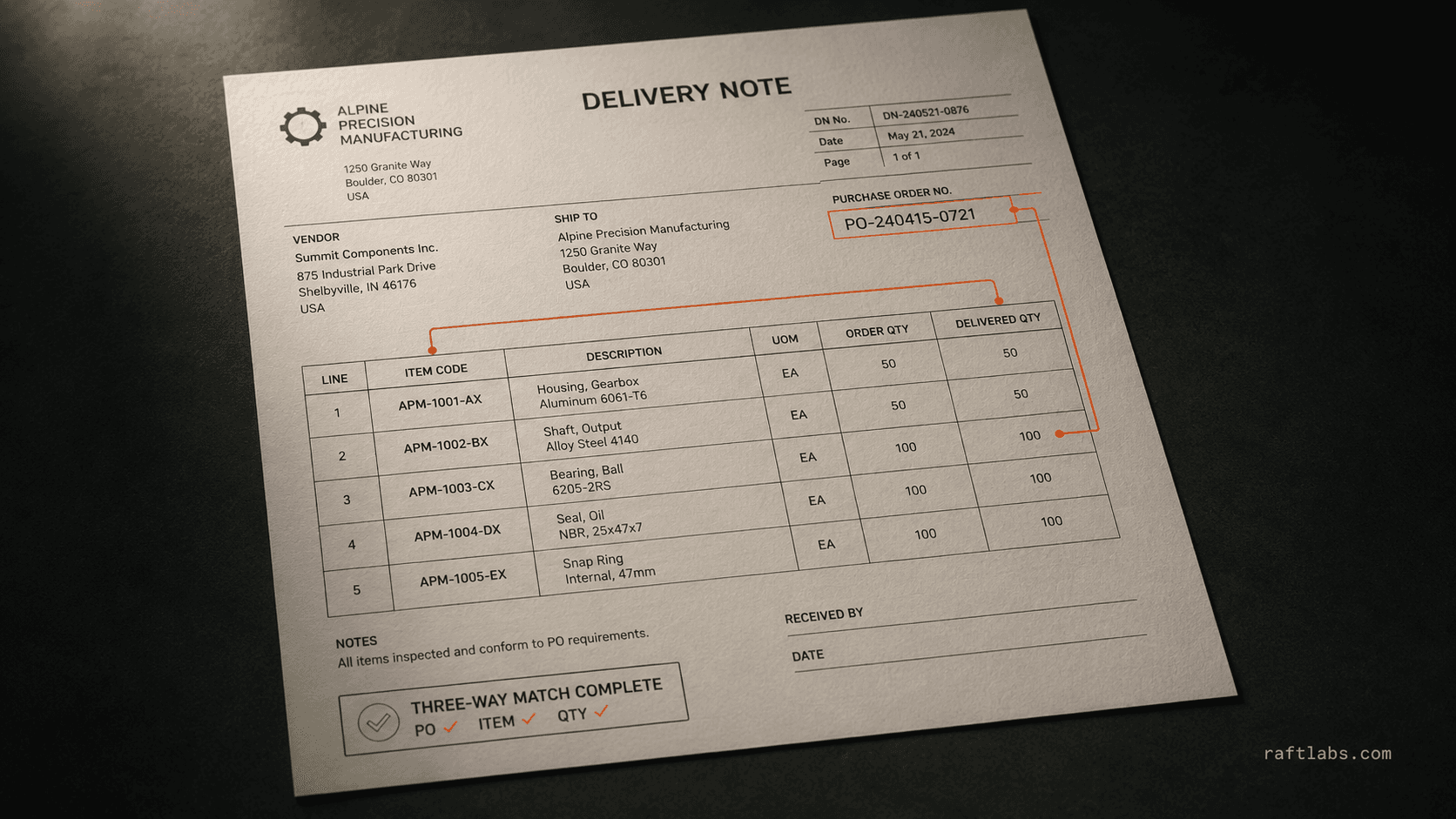
Article
Intelligent Document Processing for Manufacturing and Vendors
Intelligent document processing for manufacturing automates PO and invoice matching, maintenance logs, compliance records, and quality inspection reports.
Read more
Article
AI for energy and utilities: From reactive to predictive
Unplanned outages cost utilities $10K-$100K per hour. AI agents are catching failures weeks before they happen. The math is impossible to ignore.
Read morePredictive maintenance models for energy assets use time-series sensor data to detect the early signatures of equipment degradation before failure. For a transformer, the relevant signals include oil temperature, dissolved gas analysis readings, load current, and ambient temperature over time. For a rotating machine such as a turbine or pump, vibration frequency spectra, bearing temperatures, and oil pressure are the primary signals. The model learns the normal operating signature of each asset class and identifies deviations from that baseline that correlate with historical failure events in your maintenance records. Output is a ranked list of assets by current failure probability, the contributing sensor signals, and a recommended inspection or maintenance action. The model operates on a rolling window of sensor data, typically daily or hourly, and updates the risk ranking continuously. For assets where failure causes significant outage cost or safety risk, a 2-4 week prediction horizon gives maintenance teams enough time to plan and execute the intervention before failure occurs.
A grid demand forecasting model for distribution-level management needs historical load data at the granularity you want to forecast, typically hourly or 30-minute interval data at the feeder or substation level, going back 2-3 years. Beyond historical load, the model improves significantly with weather data: temperature is the strongest external driver of electricity demand, but humidity, wind, and solar irradiance are also relevant. Calendar features, day of week, public holidays, school terms, capture regular demand patterns that weather alone doesn't explain. For distribution utilities serving industrial customers, industrial production schedules and shift patterns are significant inputs. Output is a day-ahead or week-ahead load forecast by feeder or zone with confidence intervals. The forecasts feed procurement decisions (how much reserve to commit), dispatch scheduling, and network switching decisions. We assess your metering infrastructure and historical load data availability in discovery to determine the achievable forecast granularity and accuracy.
Pipeline anomaly detection uses the continuous sensor readings from your SCADA system, pressure at multiple points along the pipeline, flow rates, temperature, and valve positions, to detect deviations from the expected operating envelope. A baseline model learns the normal relationship between these sensor readings under different operating conditions: flow rate, ambient temperature, product type, and pressure profile. When a sensor reading or a combination of readings deviates from the predicted baseline by more than a threshold, an alert is generated. The alert includes the sensor IDs, the magnitude of the deviation, and the time window over which it developed. This is designed to surface two types of events: slow leaks that develop gradually over hours or days (a gradual pressure drop below the model's expected value for the current flow conditions) and rapid events such as a rupture or valve failure. The detection threshold is calibrated to minimize false positives, reducing alert fatigue for control room operators, while maintaining sensitivity to genuine anomalies.
Energy consumption optimization for commercial buildings uses building management system data, HVAC set points, occupancy sensors, sub-metering data by zone, and external weather, to reduce energy use while maintaining comfort targets. A model learns the thermal dynamics of the building: how long it takes to cool or heat each zone given the current weather, occupancy, and equipment settings. This allows the model to pre-cool or pre-heat a building during off-peak tariff periods rather than running HVAC at full load during peak tariff hours. For buildings with demand charges (billed on peak 15-minute demand), the model manages load across the building to shave the demand peak. For a commercial building with annual energy costs above USD 200,000, consumption optimization typically reduces energy cost by 10-20%. We assess your BMS data access and metering infrastructure in discovery.
Cost depends on the scope: a focused predictive maintenance model for a single asset class (transformers, for example) with data you already have in a historian typically runs USD 40,000-80,000 for the first build. A multi-system AI platform covering demand forecasting, anomaly detection, and field service routing for a distribution utility is a larger engagement priced in discovery. Every project is scoped at a fixed price before development starts. You see the cost breakdown, the deliverables, and the timeline in week 1 before any development begins.
Yes. We sign NDAs before any discovery conversation that involves operational data, SCADA architecture, or proprietary asset performance records. For US utilities, we are familiar with NERC CIP data handling requirements. For Australian and UK energy clients, we apply the same data classification and access controls we use for HIPAA-regulated healthcare data. Data used to train models is never retained beyond the engagement unless you explicitly authorize it.
Work with us
Bring the rough workflow, half-built product, or messy brief. We will map the smallest useful first move, then send scope, timeline, and price in plain English.